The study of the stably stratified boundary layer (SBL) is difficult because of the predominance of the local effects and the characteristics of turbulence (small scales, anisotropy and intermittency) and the Kolmogorov theory might be no longer valid.

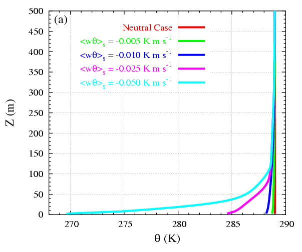
A number of numerical experiments have been performed with increasing stability of stratification to inspect until what range of stability the Kolmogorov theory for dissipation can still be used in LES of SBL (further details in Jiménez and Cuxart, 2005). The ideal simulations are made on a domain of 600×400×1431 m with 96 x 96 x 128 grid points (about 5 m resolution). Twenty different sensitivity simulations have been made. A well developed neutrally stratified turbulence field is generated for 4 different geostrophic balances G = 13, 10, 8, 5 m/s, all with potential temperature constant with height.  To study the stably stratified regime, different surface coolings were applied. It was found that the model is able to simulate from weakly to moderately stratified conditions (Figures 4.1 and 4.2). For strongly stratified conditions, the model produces a non-realistic strong surface cooling (known as runaway cooling, Figure 4.3).

In the  first GABLS LES intercomparison exercise, 11 different models were run under the same stratified conditions (Beare et al., 2006 and Figure 4.4 here). It was found that the model outputs depend on the turbulence scheme used and resolutions of about 1m are needed to properly study the stably stratified boundary layer.

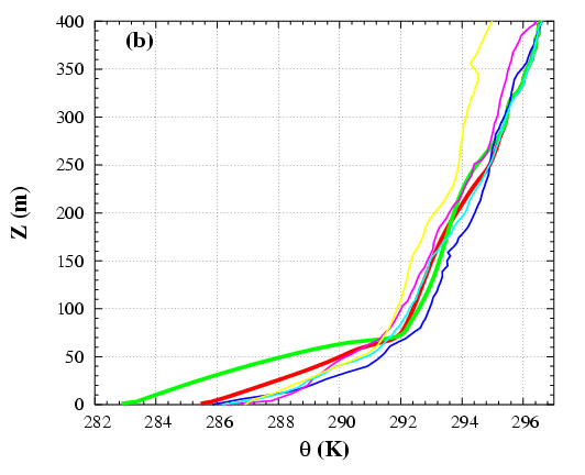
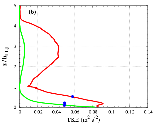
Next step was devoted to study a more realistic case with the LES. An observed Low-Level Jets (LLJ) was simulated using LES in order to study the main mechanisms present in the LLJ and the mixing across the inversion. It was found that the maximum of the wind is located at the temperature inversion (Figure 4.5). The shear above and below the jet is the responsible of the generation of turbulence whereas the buoyancy has an opposite behaviour (Figure 4.6).

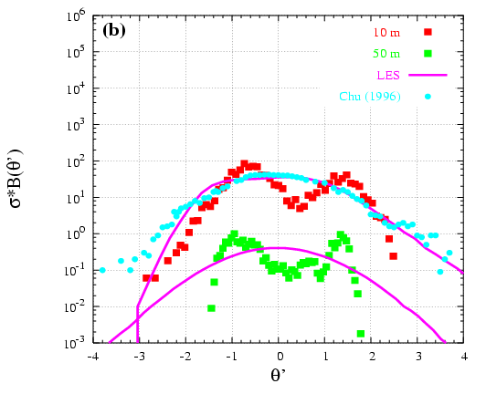
A methodoly to compare LES results and observations using Probability Density Functions is developed (Figure 4.7). It is found that the LES model is able to reproduce the main observed patterns whereas the small scale variability (far from the mean pattern) is not seen by the model.

Figure 4.1: Averaged profiles over 1h and over the horizontal for (a) potential temperature and (b) wind speed for different surface coolings.

Figure 4.2: (Left) Resolved TKE and (right) subgrid TKE over total TKE (e/E) ratio for different surface coolings.

Figure 4.3: External forcings used (points) in the LES of the shear-driven SBL case and two different criteria that specify limiting forcings that support turbulence following Derbyshire (1990). In circles simulations that suffer from runaway cooling and in triangles the rest of the runs.

Figure 4.4: Potential temperature profiles obtained from different models. (a) 6.25m resolution and (b) 2m resolution.

Figure 4.5: Half-hourly averaged LES outputs at 1h and 4h and some observed soundings (thin lines) for: (a) wind speed and (b) potential temperature

Figure 4.6: (Left) Resolved (green) and total (red) TKE obtained from the LES and (right) the observations from Sodar (the echoes at 240m indicate the presence of elevated turbulence).

Figure 4.7: Normalized PDFs for (a) wind speed and (b) potential temperature computed from data and from the LES (lines) at 10, 50, and 100 m. The PDFs at 50 and 100 m have been shifted up two and four decades, respectively, to clarify the intercomparison. PDFs obtained from data measurements in Chu et al. (1996) are shown by the open squares.